
Software
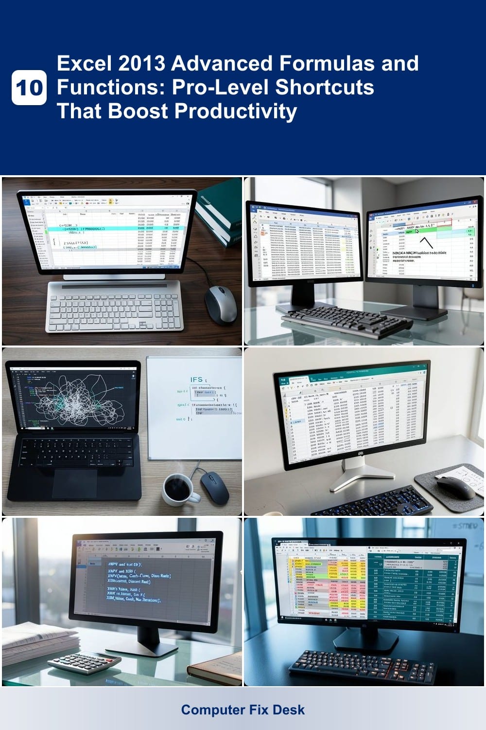
Excel 2013 remains a powerhouse for data analysis, yet many users overlook its most powerful formulas. These 10 advanced functions will transform how you manipulate data, automate tasks, and uncover insights—without requiring VBA coding.
Array Formulas for Dynamic Data Analysis
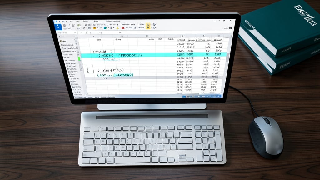
Tired of cluttering your spreadsheets with helper columns just to perform multi-cell calculations? Array formulas in Excel 2013 let you perform complex operations—like summing ranges or multiplying values—across entire columns or rows without extra cells, making your workbooks cleaner and more dynamic.
To use them, simply enter your formula (e.g., {=SUM(A1:A10*B1:B10)}) and press Ctrl+Shift+Enter to create an array. Excel 2013 will surround it with curly braces {} automatically. These formulas excel in financial modeling (e.g., calculating weighted averages) or dynamic reporting where ranges frequently expand. For example, {=AVERAGEIF(A1:A100,">50")} returns the average of all values over 50 in a single step.
Perfect for accountants, analysts, or anyone crunching numbers where helper columns slow you down. Just remember: Excel 2013 requires the Ctrl+Shift+Enter shortcut—no need for VBA! ✨
Advanced Lookup with INDEX MATCH
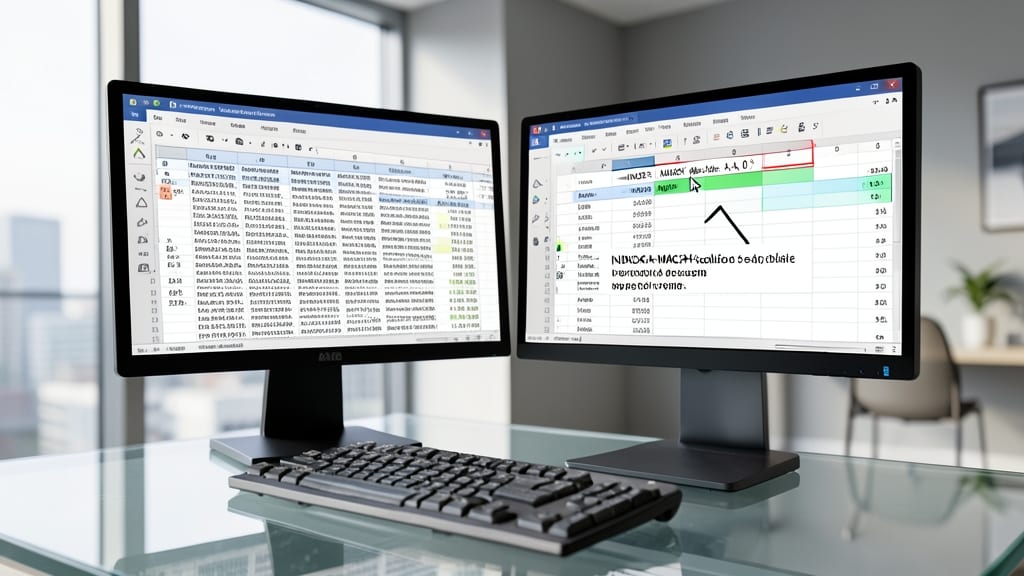
Tired of VLOOKUP breaking when your dataset rearranges? The INDEX-MATCH combo is your upgrade—it retrieves data without requiring sequential columns, making it perfect for real-world datasets with irregular structures.
Here’s how it works: MATCH finds the position of your lookup value (anywhere in the row), while INDEX pulls the exact cell you need. For example, =INDEX(B2:B100, MATCH("Apple", A2:A100, 0)) returns the price of "Apple" even if it’s not the first column. No more #N/A errors from misaligned data!
This is a game-changer for inventory managers or analysts dealing with merged datasets or pivot table outputs. Once mastered, you’ll wonder how you ever relied on VLOOKUP. ✨
Conditional Logic with IFS Function

Tired of tangled IF statements that stretch across your Excel sheet like a tangled power cord? The IFS function in Excel 2013 lets you stack multiple conditions into a single, clean formula—no more nesting headaches.
With IFS, you test up to 127 conditions in one line, each paired with a corresponding value. For example, an HR payroll system could assign bonuses with:
=IFS(A2="A", 1000, A2="B", 500, A2="C", 250)
No more IF(AND(OR(...))) chaos. It also auto-stops at the first true condition, saving calculation time.
Perfect for HR departments, financial analysts, or anyone managing tiered decision workflows. Your spreadsheets will thank you. ✨
Text Manipulation with TEXTJOIN and TEXTSPLIT
Tired of manually cleaning messy text data in Excel 2013? TEXTJOIN and TEXTSPLIT let you combine or divide text dynamically—no helper columns required. These functions are game-changers for importing CSV files or generating custom reports where text formatting is inconsistent.
TEXTJOIN merges text from multiple cells with a delimiter (like commas or spaces) while ignoring empty cells, while TEXTSPLIT breaks text into columns based on a delimiter. Both work in Excel 2013 without needing Power Query or VBA. For example, =TEXTJOIN(", ", TRUE, A1:A10) combines all values in A1:A10 with a comma separator, skipping blanks.
Perfect for data analysts, marketers, or anyone wrestling with exported datasets. Say goodbye to manual copy-pasting and hello to zero-config text cleanup. ✨
Financial Modeling with XNPV and XIRR

When cash flows arrive at unpredictable intervals, XNPV and XIRR in Excel 2013 become your secret weapon for precise financial analysis. Unlike NPV or IRR—designed for regular intervals—these functions account for real-world timing, ensuring your projections reflect actual investment scenarios.
XNPV calculates net present value for irregular cash flows using discount rates and exact dates, while XIRR computes the internal rate of return for the same irregular schedule. For example, if you’re evaluating a project with payments on January 15, March 20, and June 5, these functions deliver results that match real-world timing—unlike standard NPV or IRR, which assume equal intervals.
Investors and accountants rely on these to assess project viability, compare investment options, or audit financial reports. If you’re working with real-time data where timing matters, these functions save hours of manual adjustments. ✨
Data Validation with AGGREGATE Function
Frustrated when volatile functions like STDEV or AVERAGE recalculate endlessly and break your reports? The AGGREGATE function in Excel 2013 gives you full control—ignoring errors, hidden rows, or even specific calculations entirely, so your quality control reports stay rock-solid.
With AGGREGATE, you specify which function to use (e.g., 1 for AVERAGE, 2 for COUNT, 6 for STDEV) and how to handle errors or hidden data via the ignorehidden or ignoreerror options. For example, =AGGREGATE(6,5,A1:A100) calculates standard deviation while ignoring errors, while =AGGREGATE(9,6,A1:A100) sums visible cells only—no more #DIV/0! surprises.
Perfect for quality control analysts or manufacturing teams where data integrity is critical. This function turns volatile calculations into reliable, error-proof metrics. ⚡
Dynamic Range Handling with OFFSET and INDIRECT
Tired of manually resizing ranges every time your monthly sales data expands? The OFFSET and INDIRECT combo lets you create self-adjusting ranges that grow with your data—no manual updates needed.
Use OFFSET to define a starting cell and dynamically adjust the range size (e.g., =OFFSET(A1,0,0,COUNTA(A:A),1)), then wrap it in INDIRECT to reference it flexibly. This is perfect for pivot tables or dashboards where data sources like Excel Tables or imported CSV files change monthly. Combine them with SUM or AVERAGE to keep calculations current effortlessly.
Accountants and operations managers will love this for automated financial reports, while analysts can use it to build self-updating dashboards without VBA. ⚡
Statistical Analysis with PERCENTRANK and QUARTILE
Tired of manually sorting data to find percentiles or quartiles? PERCENTRANK and QUARTILE in Excel 2013 automate this process instantly—no sorting required. These functions reveal how your data compares to industry benchmarks or market trends without tedious manual calculations.
PERCENTRANK tells you where a specific value falls within a dataset (e.g., "This sales figure is in the 85th percentile"), while QUARTILE divides data into four equal parts (Q1, Q2, Q3, Q4). Both work with Excel Tables or ranges, and handle ties automatically. For example, QUARTILE(A2:A100, 2) instantly returns the median value, while PERCENTRANK(A2:A100, 50) shows where 50 sits in the distribution.
Perfect for analysts in market research, operations, or finance who need to benchmark performance against peers or historical data. ⚡
Error Handling with IFERROR and ISERROR
Tired of seeing #DIV/0! or #VALUE! errors crash your polished reports? IFERROR and ISERROR are your secret weapons for turning ugly errors into clean, professional outputs—no VBA required.
Use IFERROR to replace errors with custom messages (e.g., =IFERROR(A1/B1, "N/A")) or fallback values. ISERROR lets you test for errors first, then handle them with logic like =IF(ISERROR(A1), "Invalid", A1). Both work in Excel 2013 and preserve calculation speed, making them ideal for dashboards shared with non-technical teams.
Accountants, sales analysts, and project managers will love these for user-facing reports where errors would otherwise derail credibility. ⚡
Date Calculations with EOMONTH and WORKDAY

Tired of manually adjusting dates in Excel to account for weekends or month-end deadlines? The EOMONTH and WORKDAY functions automate these tasks effortlessly—perfect for operations teams managing logistics or project timelines.
EOMONTH returns the last day of a month based on a start date and offset (e.g., =EOMONTH("5/15/2023", 2) gives July 31, 2023). Meanwhile, WORKDAY adds business days while excluding weekends and holidays (e.g., =WORKDAY("5/1/2023", 10, A2:A5) skips weekends and custom holidays in range A2:A5). Both functions work seamlessly in Excel 2013 without macros.
Logistics coordinators and project managers will love these for scheduling deliveries or tracking deadlines—no more guesswork! ✨